Nomad Cyclist Problem - Ancient Silk Road on Bicycle
An step by step guide to Traveling Salesman Problem and it’s application in cycle tour planning
Silk Road is an ancient network of routes encompassing dozens of cities in Western China, Central, West and South Asia. In the past, there were no roads for ancient traders and travelers to travel on. The shortest known path from a city to another city usually became part of the route. Exceptions were made in order to avoid thugs, tough weather and the risk of running out of food and water.
A few friends of mine are planning a bicycle tour through the ancient Silk Road next year. This is going to be a human powered trip similar to how most people traveled through these routes in old times. My friends are not pro-cyclists. So, every paddle must be stroked in the right direction in this journey of thousands of Kilometers.
I initially thought it’s a crazy idea but then I realized it is going to be a trip of a lifetime. So, I decided to give programming a try to plan the tour.
Cities
These cyclists have planned that the following major ancient cities cannot be missed on the Silk Road:
Xi’an, China 🇨🇳 (origin place of silk trade)
Lanzhou, China 🇨🇳
Dunhuang, China 🇨🇳
Gaochang, China 🇨🇳
Urumqi, China 🇨🇳
Almaty, Kazakhstan 🇰🇿
Bishkek, Kyrgyzstan 🇰🇬
Tashkent, Uzbekistan 🇺🇿
Dushanbe, Tajikistan 🇹🇯
Baysun, Uzbekistan 🇺🇿
Samarkand, Uzbekistan 🇺🇿
Bukhara, Uzbekistan 🇺🇿
Merv, Turkmenistan 🇹🇲
Ashgabat, Turkmenistan 🇹🇲
Tehran, Iran 🇮🇷
Tabriz, Iran 🇮🇷
Ankara, Turkey 🇹🇷
Istanbul, Turkey 🇹🇷
There are cities along the route that are very rich in historical sites and have significance in the ancient trade but it is not possible to include all of them in a human powered bicycle tour. For example, Taxila in Pakistan and Kashgar in China.
Traveling Salesman problem
In order to find a shortest route through all of these cities, let’s use the classic Traveling Salesman Problem (hereafter TSP) algorithm. TSP is an optimization problem. TSP says
“Given a list of cities to visit and distances between each of them, what is the shortest path to visit all these locations and return back to our starting location”
In the original TSP, the route we calculate is a closed route and our start and end locations must be the same.
But as cyclists, we are interested in visiting the cities on our way, we are not interested in going back to the starting location. TSP has many variations, let’s call this variation of TSP as “Nomad Cyclist Problem”.
Distance Matrix
Distance Matrix is the starting point to formulating almost any optimization problem involving a path. E.g. Shortest Path Problem, Traveling Salesman Problem, Vehicle Routing Problem and Route Optimization for logistics.
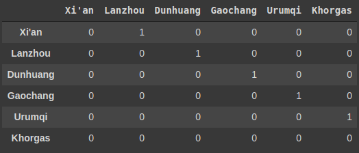
Have a look at the following Distance Matrix:
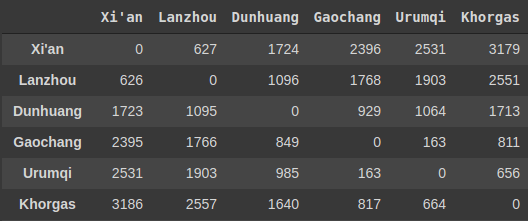
The cell in 2nd row and 1st column has value 626. This is the distance in kilometers from Lanzhou to Xi’an. The distance from Xi’an to Lanzhou however, is 627 indicated by the cell in the first row’s 2nd column.
The value of each cell in the above table is the length of the road in kilometers, from the city on the left to the city in the top header.
We will use a 2D array (or a 2D list in Python) to store Distance Matrix values.
# distance matrix
D = [[0, 627, 1724, 2396, 2531, 3179],
    [626, 0, 1096, 1768, 1903, 2551],
    [1723, 1095, 0, 929, 1064, 1713],
    [2395, 1766, 849, 0, 163, 811],
    [2531, 1903, 985, 163, 0, 656],
    [3186, 2557, 1640, 817, 664, 0]]
For real world locations, we can easily calculate the distance matrix for our locations using Google Maps Distance Matrix API and Mapbox’s Matrix API using simple API calls.
Compute Distance Matrix
Calculating distance matrix by hand for more than a couple of cities becomes tiresome. Let’s write some scripts to compute the distance matrix for us.
To compute the distance matrix using Google Maps Matrix API, we can simply provide the name of the places. But I decided to hardcode longitude, latitude coordinates of the cities. I think coordinates avoid confusion when more than one place has a similar name.
The getCities method gives a list of cities + coordinates.
def getCities():
    # locations to visit
    cities = [
        {
            "name": "Xi'an, Shaanxi, China",
            "location": [34.341576, 108.939774]
        },
        {
            "name": "Lanzhou, China",
            "location": [36.061089, 103.834305]
        },

        ...

        {
            "name": "Istanbul, Turkey",
            "location": [41.022576, 28.961477]
        }
    ]
    return cities
Compute Distance Matrix
Computing the Distance Matrix is easy now. We just have to call a gmap API endpoint, provide the two lists: origins & destinations, between which we want to compute distances and get back our distance matrix as JSON that will be parsed and converted into a 2D list D we saw above.
import requests, traceback

def gmapMatrix(origins, destinations):
    API_KEY = GET_GMAP_API_KEY() # <<= put your gmap api key
    URL = f"https://maps.googleapis.com/maps/api/distancematrix/json?units=metric&origins={origins}&destinations={destinations}&key={API_KEY}"

    try:
        r = requests.get(URL)
        jsn = r.json()

        return jsn
    except Exception:
        traceback.print_exc()
        return None
Let’s find our distance matrix. Welp, not so easy. It turns out Google’s Matrix APIs has a few limits.
According to Google Maps Matrix API:
- “Each query sent to the Distance Matrix API generates elements, where the number of origins times the number of destinations equals the number of elements.”
- Maximum of 25 origins or 25 destinations per request are allowed
- Maximum 100 elements per server-side request are allowed
Compute Distance Matrix for more than 100 elements
We have about 20 cities. 20*20 equals 400. We are above the 100 elements limit. We have to divide our request in batches of 100, fetch the distances and construct our 20 x 20 distance matrix.
If you are familiar with Convolutional Neural Networks in Deep Learning, you might know the convolution technique in which we take a small part of matrix, do some operation and calculate another matrix. This process is step by step and works on a small part of the matrix at a time.

Don’t worry, our calculations for takling the 100 elements limit are much simpler than Convolutional Neural Nets.
Take a look at convolveAndComputeDistMatrix method in the project code. This method goes over the distance matrix, picks only 100 items to find distance and constructs a distance matrix of 20 x 20… our desired Distance Matrix.
Implementation
Let’s formulate our Nomad Cyclist Problem (TSP) as a Linear Programming problem. To solve an Linear Programming problem, we usually need 4 things
- Decision Variables
- Constraints
- Objective
- Solver
Solver
A (optimization) solver is a software or library which takes an optimization problem defined (modeled) in a certain way and tries to find an optimum solution to that problem. Our job is to model the problem properly, the solver does the heavy duty.
We will use OR-Tools which is an open source library by Google AI team for tackling optimization problems.
Let’s see how to model our problem for OR-Tools Initialize OR-Tools’ Linear Solver
from ortools.linear_solver import pywraplp

s = pywraplp.Solver('TSP', pywraplp.Solver.GLOP_LINEAR_PROGRAMMING)
Decision Variable
In simple words, decision variables are the variables that will contain the output of the Linear Programming algorithm. The decision made by our algorithm!
For TSP, a decision variable will be a 2D list of the same size as Distance Matrix. It will contain 1 in the cells whose corresponding roads must be visited and hence part of the output route. And 0 at roads that must not be traveled.
According to OR-Tools Linear Solver documentation, we define an integer decision variable using IntVar.
So, let’s say we want to create a variable named count that will hold the number of times a certain task is done. We will probably start it with 0 and will keep incrementing with each task until the end of our program, where it would contain some useful value of our interest.
count = 0
If we want to define the same variable but to be used by the OR-Tools Linear Solver, we will define it as follows (and it will now be called a decision variable).
# IntVar(lowerBound, upperBound, name)
count = solver.IntVar(0, 100, 'count_var')
Notice that we have to provide bounds too. This tells the solver to find an integer value that is from lowerBound to upperBound. This helps narrow down the possible outputs and the solver can find the solution faster.
Now we define our decision variable for TSP. It is going to be a 2d Python list of IntVars. But here, the bounds of cities will be 0 to 1 except for the cities whose inner distances were not found, for them bounds will be 0 to 0.
x = [[s.IntVar(0, 0 if D[i][j] is None else 1, '') \
        for j in range(n)] for i in range(n)]
Constraints
Think of constraints as the limits or rules that must be respected. According to TSP,
“We must visit every city in a single closed path exactly once.”
First we will solve TSP for a closed tour. Then we’ll modify it to give an open shortest path for our Nomad Cyclists. So, in our solution there must be only one road (used for) going to a city and only one road going out of the city.
for i in range(n):
    # in i-th row, only one element can be used in the tour
    # i.e. only 1 outgoing road from i-th city must be used in the tour
    s.Add(1 == sum(x[i][j] for j in range(n)))

    # in j-th column, only one element can be used in the tour
    # i.e. only 1 incoming road to j-th city must be used in tour
    s.Add(1 == sum(x[j][i] for j in range(n)))

    # a city must not be assigned a path to itself in the tour
    # no direct road from i-th city to i-th city again must be taken
    s.Add(0 == x[i][i])
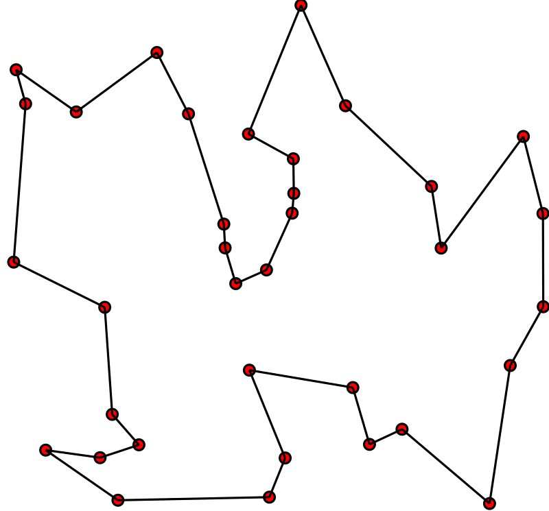
The above constraints are not enough. There are sometimes problematic subtours and each of them covers a subset of distinct cities but none of them cover all the cities. We want one (shortest) tour through all cities.
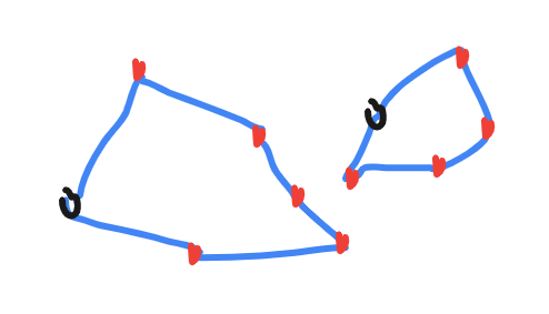
We know that any closed path consisting of 6 cities has 6 arcs (edges / roads) connecting them (like above photo). So, we tell our solver that if a tour is a subtour (i.e. it covers cities less than total cities in distance matrix) the roads connecting these cities must be less than the number of cities in this subtour. This will enforce the solver to find subtours that are not closed, which will eventually lead to successfully finding a closed (shortest) tour connecting all cities.
But we cannot find all possible subtours and include them in our constraint. A way to avoid such subtours is that on the first run of our algorithm, we find a solution and if it consists of subtours, we run the algorithm again and this time we tell it to keep those subtours unclosed. We keep repeating the process until we find a single optimal tour that covers all cities instead of small disconnected subtours.
Let’s model this constraint:
# Subtours from previous run (if any)
for sub in Subtours:
    # list containing total outgoing+incoming arcs to
    # each city in this subtour
    K = [ x[sub[i]][sub[j]] + x[sub[j]][sub[i]] \
         for i in range(len(sub)-1) for j in range(i+1,len(sub)) ]

    # sum of arcs (roads used) between these cities must
    # be less than number of cities in this subtour
    s.Add(len(sub)-1 >= sum(K))
Objective
The goal of our Integer Programming algorithm. In our case, we want to minimize the distance we have to cover to visit all the cities.
# minimize the total distance of the tour
s.Minimize(s.Sum(x[i][j]*(0 if D[i][j] is None else D[i][j]) \
                   for i in range(n) for j in range(n)))
In other words, find a route through these cities that is a shortest path, while respecting the above constraints. It is ‘a’ shortest path. Because there can be multiple shortest paths of same the length.
Nomad Cyclist Problem
TSP with an open route will be our Nomad Cyclist Problem. A simple trick to make our existing algorithm find an open route instead of a closed one is to add a dummy city to the distance matrix. Set the distance of this dummy city to 0 from all the other cities.
When the solver will find the optimum solution, there will be this dummy city somewhere along the closed route. We simply delete this dummy city and it’s incoming & outgoing arcs (roads) to get an open route for our Nomad Cyclists.
# to make the loops run 1 more time then current size of our lists
# so we could add another row / column item
n1 = n + 1

# if i or j are equal to n, that means we are in the last row / column
# just add a 0 element here
E = [[0 if n in (i,j) else D[i][j] \
    for j in range(n1)] for i in range(n1)]
The resulting route will be the shortest one way and open tour covering all the cities.
Manual v Calculated tour comparison
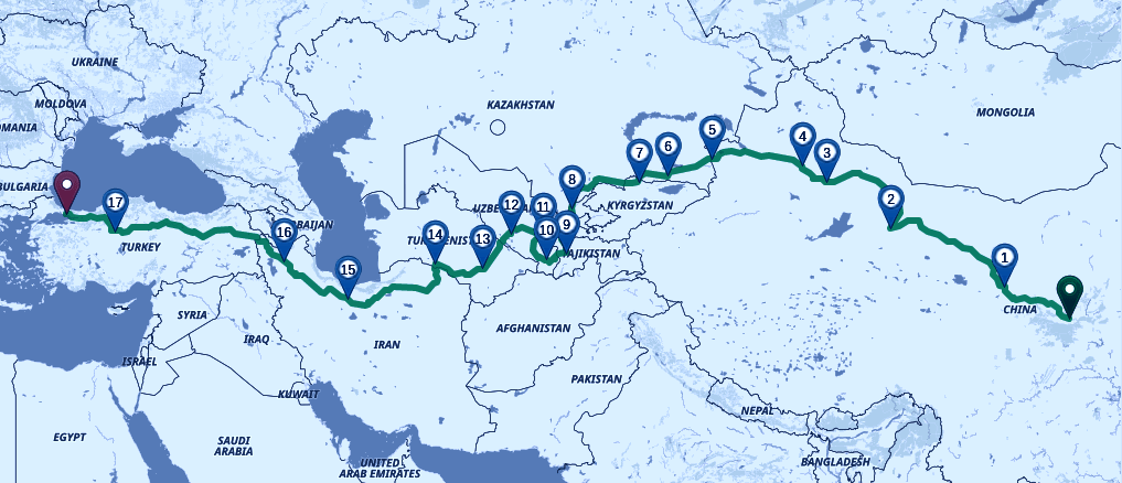
According to our solver, we must cycle through cities in this order
Shortest Path for our Cycling Tour:
    Cities:  Xi'an  Lanzhou  Dunhuang  Gaochang  Urumqi  Khorgas  Horgos  Almaty  Bishkek  Tashkent  Samarqand  Dushanbe  Baysun  Bukhara  Merv  Ashgabat  Tehran  Tabriz  Ankara  Istanbul
 City Index      0        1         2         3       4        5       6       7        8         9         12        10      11       13    14        15      16      17      18        19
   Distance      0      627      1096       929     163      656      -1     332      237       631        310       292     196      341   353       400     948     632    1463       451
 Cumulative      0      627      1723      2652    2815     3471    3470    3802     4039      4670       4980      5272    5468     5809  6162      6562    7510    8142    9605     10056
A photo of same output in case the above output does not appear readable:

After deciding the cities to visit, we made a rough plan about the order in which we will visit these places. On Google Maps, you cannot create a route between more than 10 places (I think).
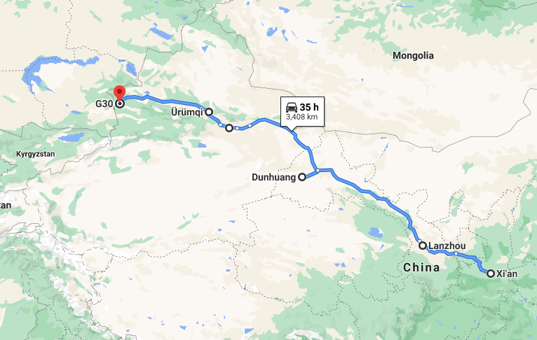
First leg of our previously planned route for Chinese Silk Road cities, which matches the route suggested by our algorithm:
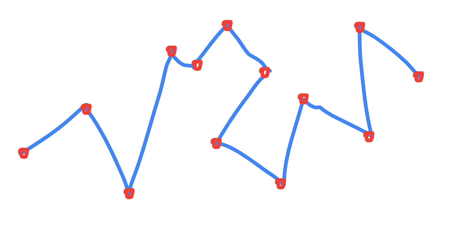
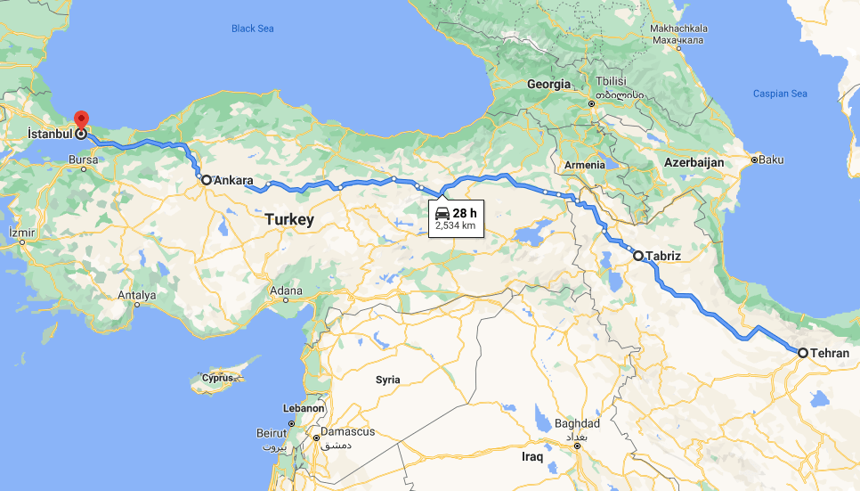
Last leg of our planned tour through the Middle East to Europe… this also matches with algorithm output:
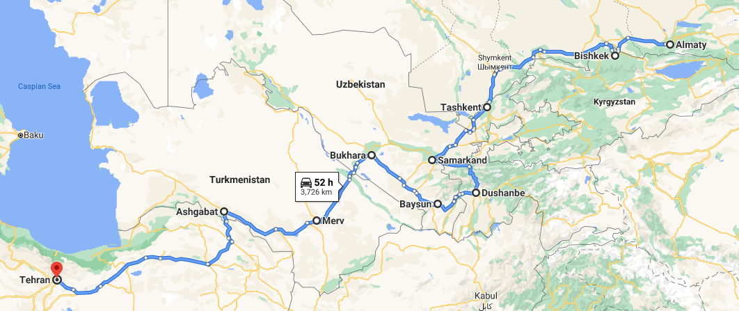
2nd (center) leg of our manually planned route for Central Asian cities:
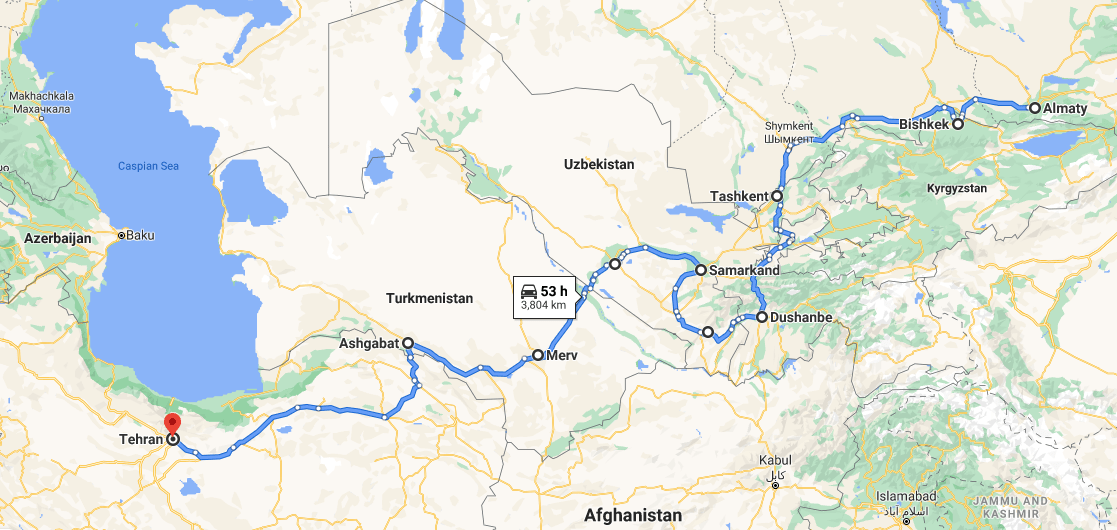
The shortest route by our algorithm matches about 90% of our manually planned route except a few cities in Central Asia:
When cycling thousands of kilometers, even a couple hundred kilometers less traveled to reach our destination feels like a relief. We hope this has been a great guide to the Traveling Salesman Problem and Nomad Cyclist Problem. An important thing we’ll consider next is the elevation.
Plan your own route
All the project code is on GitHub as Nomad Cyclist and is full of helpful comments. Feel free to customize it and make a pull request.
The (TSP) Linear Programming algorithm used here is taken from Serge Kruk’s Practical Python AI Projects book. Highly recommended if you want to study route optimization algorithms or optimization algorithms in general.
Next, we will be adding the option to consider elevation and climb difficulty too, a very important thing to consider for cyclists while planning tours.